Mastering the VLOOKUP Function

In this article, you will learn how to effectively use the VLOOKUP function to enhance your skills in Excel. We will walk you through the step-by-step process of creating a VLOOKUP formula, and explain the syntax and parameters involved. By the end of this article, you will have a solid understanding of how to use the VLOOKUP function to search for and retrieve specific information from a table or range. So, let’s get started on mastering the VLOOKUP function together!

Mastering the VLOOKUP Function

If you have ever worked with spreadsheets in Microsoft Excel, you have probably come across the VLOOKUP function. VLOOKUP, which stands for “Vertical Lookup,” is a powerful tool that allows you to search for a specific value in a dataset or range and retrieve related information from another column or sheet. It is one of the most commonly used functions in Excel and is a valuable skill to have for anyone who works with data.

Definition of VLOOKUP

VLOOKUP is a built-in function in Excel that helps you find values in a table by looking up a specified value in the leftmost column of that table. Once the value is found, you can retrieve information from any column to the right of the lookup column. This function is useful for tasks such as searching for employee details, calculating grades, or creating dropdown menus.

Benefits of using VLOOKUP

There are several benefits to using the VLOOKUP function in Excel:

1. Efficiency: VLOOKUP allows you to quickly search for and retrieve information from large datasets without the need for manual searching or filtering.

2. Accuracy: With VLOOKUP, you can be confident that you are retrieving the correct information, as long as your lookup value and table are set up correctly.

3. Flexibility: VLOOKUP can be used for both exact and approximate matches, giving you the flexibility to search for values that are not an exact match.

Now that we understand the basics of VLOOKUP, let’s delve into its syntax and parameters.

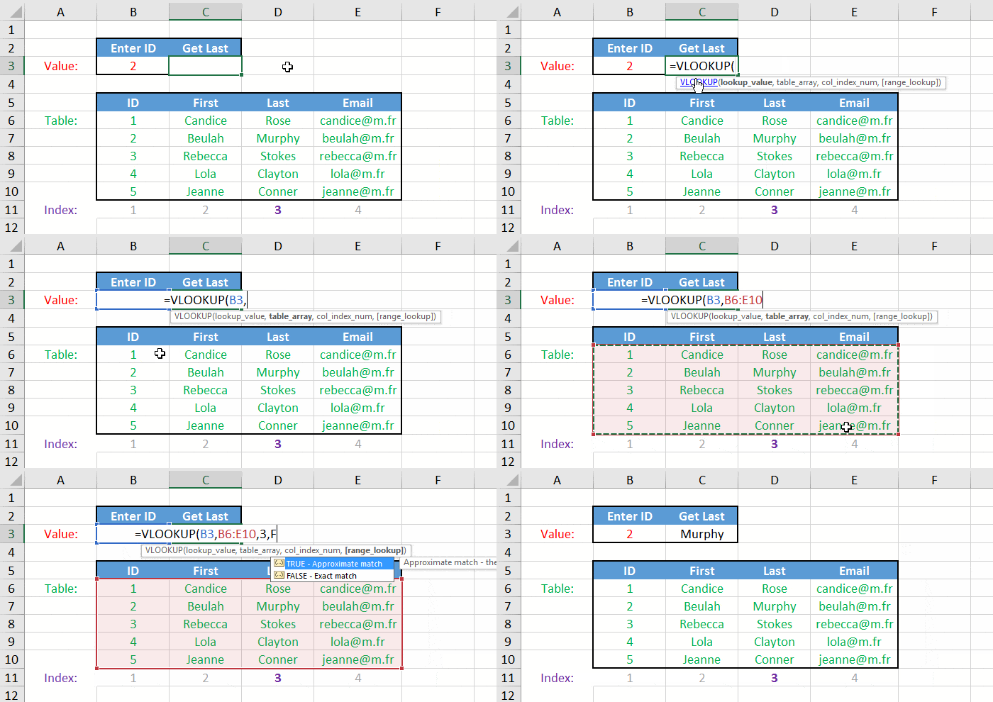
Understanding the Syntax of VLOOKUP

The syntax of the VLOOKUP function is as follows:

=VLOOKUP(lookup_value, table_array, col_index_num, [range_lookup]) 

Parameters of VLOOKUP

• lookup_value: This is the value you want to search for in the leftmost column of the table.
• table_array: This is the range of cells that contains the data you want to search in. It should include both the lookup column and the columns from which you want to retrieve information.
• col_index_num: This is the column number from which you want to retrieve information. The leftmost column in the table is considered column 1.
• range_lookup: This is an optional parameter that indicates whether you want an exact or approximate match. If set to TRUE or omitted, VLOOKUP will search for an approximate match, and if set to FALSE, it will search for an exact match.

How to choose the correct range for VLOOKUP

It is essential to choose the correct range for VLOOKUP to ensure accurate results. The table_array should cover all the data you want to search in and include both the lookup column and the columns from which you want to retrieve information. If you omit any columns from the range, VLOOKUP will not be able to retrieve information from those columns.

Additionally, it is crucial to ensure that the lookup column is the leftmost column in your table_array. VLOOKUP searches for the lookup value in the leftmost column and retrieves information from columns to the right.

Now that we understand the syntax and parameters of VLOOKUP, let’s learn how to use it to search for values.

Using VLOOKUP to Search for Values

How to use VLOOKUP to find an exact match

To use VLOOKUP to find an exact match, follow these steps:

1. Enter the VLOOKUP formula in the cell where you want to display the result.
2. Specify the lookup_value, table_array, and col_index_num parameters in the formula.
3. Set the range_lookup parameter to FALSE or omit it if you want an exact match.
4. Press Enter to calculate the formula and retrieve the result.

For example, if you have a table with employees’ names in column A and their IDs in column B, you can use VLOOKUP to find the ID of a specific employee by searching for their name.

=VLOOKUP("John Doe", A:B, 2, FALSE) 

This formula will search for “John Doe” in column A and retrieve the corresponding ID from column B.

Steps to perform a VLOOKUP for an approximate match

To perform a VLOOKUP for an approximate match, follow these steps:

1. Sort the lookup column in ascending order to ensure accurate results.
2. Enter the VLOOKUP formula in the cell where you want to display the result.
3. Specify the lookup_value, table_array, and col_index_num parameters in the formula.
4. Set the range_lookup parameter to TRUE or omit it if you want an approximate match.
5. Press Enter to calculate the formula and retrieve the result.

For example, if you have a table with product prices in column A and corresponding quantities in column B, you can use VLOOKUP to find the quantity of a specific product based on its price.

=VLOOKUP(25, A:B, 2, TRUE) 

This formula will search for the closest match to the price of 25 in column A and retrieve the corresponding quantity from column B.

Now that we have covered the basics of using VLOOKUP, let’s explore some common errors and error handling techniques.

Dealing with Errors in VLOOKUP

As with any function in Excel, VLOOKUP can produce errors in certain situations. Understanding these errors and knowing how to handle them is crucial to ensure the accuracy of your results.

Common errors in VLOOKUP

Some common errors you may encounter when using VLOOKUP are:

1. #N/A: This error occurs when VLOOKUP cannot find the lookup_value in the lookup column. It can happen due to a misspelled value or if the value does not exist in the dataset.

2. #REF!: This error occurs when the range_lookup parameter is set to FALSE, and the lookup_value is smaller than the smallest value in the lookup column or larger than the largest value.

3. #VALUE!: This error occurs when the lookup_value is not a valid value, such as text instead of a number.

Error handling techniques

To handle errors in VLOOKUP, you can use various techniques:

1. IFERROR function: The IFERROR function allows you to specify a value or action to take if an error occurs. You can wrap your VLOOKUP formula with the IFERROR function to display a custom message or value instead of the error.

=IFERROR(VLOOKUP(lookup_value, table_array, col_index_num, [range_lookup]), "Not Found") 

In this example, if the VLOOKUP function produces an error, the message “Not Found” will be displayed instead.

2. Error checking: Excel provides error checking tools that can help you identify and fix errors in your VLOOKUP formulas. These tools highlight cells with errors and provide suggestions for resolving them.

3. Data validation: Implementing data validation techniques, such as dropdown menus or input restrictions, can prevent errors by limiting the possible values that users can enter.

Now that we have covered error handling, let’s explore some advanced techniques that can enhance your VLOOKUP skills.

Advanced Techniques with VLOOKUP

While VLOOKUP is a powerful function on its own, combining it with other functions can further extend its capabilities. Let’s explore some advanced techniques you can use with VLOOKUP.

Combining VLOOKUP with other functions

You can combine VLOOKUP with other functions to perform complex calculations or retrieve specific information based on multiple criteria.

For example, you can use the CONCATENATE function to combine the results of multiple VLOOKUP formulas and create a custom output. Suppose you have a table with employee names in column A and their respective departments in column B. You can use the following formula to create a list of employees in a specific department:

=CONCATENATE(IFERROR(VLOOKUP("Sales", A:B, 1, FALSE), ""), ",", IFERROR(VLOOKUP("Sales", A:B, 1, TRUE), "")) 

This formula will search for the department “Sales” in column B and create a comma-separated list of employees’ names.

Using VLOOKUP with wildcards for flexible searches

By incorporating wildcards into your VLOOKUP formulas, you can perform flexible searches and retrieve information based on partial matches.

The wildcard character “?”, which represents any single character, and the wildcard character “*”, which represents any sequence of characters, can be used with VLOOKUP.

For example, suppose you have a table with product names in column A, and you want to retrieve the price of a product based on a partial match. You can use the following formula:

=VLOOKUP("*apple*", A:B, 2, FALSE) 

This formula will search for any product name that contains the word “apple” and retrieve the corresponding price from column B.

Performing multiple VLOOKUPs with INDEX and MATCH

In some cases, you may need to perform multiple VLOOKUPs to retrieve information from different columns or sheets. Instead of nesting multiple VLOOKUP functions, you can use the combination of INDEX and MATCH functions.

The MATCH function helps you find the position of a value in a range, and the INDEX function retrieves the value from that position.

For example, suppose you have a table with customer names in column A, and you want to retrieve their addresses and contact numbers from different columns. You can use the following formula:

=INDEX(B:C, MATCH("John Doe", A:A, 0), 0) 

This formula will search for the name “John Doe” in column A and retrieve the corresponding address and contact number from columns B and C.

By combining VLOOKUP with other functions, you can unlock the full potential of Excel and perform advanced data analysis tasks. Now, let’s move on to some tips and tricks for efficient VLOOKUP usage.

Tips and Tricks for Efficient VLOOKUP Usage

While VLOOKUP is a powerful function, there are some tips and tricks that can help you maximize its efficiency and make your work with Excel more productive. Let’s explore some of these tips and tricks.

Sorting data for better VLOOKUP performance

Sorting your data before using VLOOKUP can significantly improve its performance. When the data is sorted, Excel can use a binary search algorithm to find the lookup value more efficiently.

To sort your data, select the range you want to sort, go to the Data tab, and click on the Sort button. Choose the column you want to sort by and the sorting order (ascending or descending). Once the data is sorted, you can use VLOOKUP with better performance.

Utilizing named ranges with VLOOKUP

Named ranges can make your VLOOKUP formulas more readable and easier to understand, especially when working with large datasets or complex formulas. Instead of referring to cell references, you can assign names to specific ranges of cells.

To create a named range, select the range of cells you want to name, go to the Formulas tab, and click on the Define Name button. Enter a name for the range and click OK. Once you have named your range, you can use the name instead of cell references in your VLOOKUP formula.

=VLOOKUP("John Doe", Employees, 2, FALSE) 

In this example, “Employees” is the name assigned to the range containing the employee names and IDs.

Quickly copying VLOOKUP formulas to multiple cells

If you need to apply the same VLOOKUP formula to multiple cells, you can save time by using the autofill handle.

Simply enter your VLOOKUP formula in the first cell, select the cell, and grab the fill handle (a small square in the lower-right corner of the cell). Drag the fill handle across the range of cells where you want to apply the formula. Excel will automatically adjust the formula for each cell, updating the references accordingly.

Now that we have explored some tips and tricks for efficient VLOOKUP usage, let’s move on to practical examples of how VLOOKUP can be applied in various scenarios.

Practical Examples of VLOOKUP

VLOOKUP can be used in a wide range of real-life scenarios. Let’s take a look at some practical examples of how VLOOKUP can be applied.

VLOOKUP to retrieve employee details from a database

Suppose you have a database of employee details with columns for employee names, IDs, departments, and salaries. You can use VLOOKUP to retrieve specific information based on an employee’s name or ID.

For example, if you want to find the salary of an employee with the ID “1001,” you can use the following formula:

=VLOOKUP("1001", A:D, 4, FALSE) 

This formula will search for the ID “1001” in column A and retrieve the salary from column D.

Calculating grades using VLOOKUP

If you are a teacher or involved in the education sector, VLOOKUP can help you automate the process of calculating grades based on scores or percentages.

Suppose you have a table with score ranges and corresponding grade letters. You can use VLOOKUP to find the grade based on a student’s score.

=VLOOKUP(B2, ScoreTable, 2, TRUE) 

In this example, the student’s score is in cell B2, and “ScoreTable” is the named range that contains the score ranges and grade letters.

Creating dropdown menus with VLOOKUP

Dropdown menus can make data entry more user-friendly and prevent errors. You can use VLOOKUP to create dropdown menus that are based on a list of values in a separate column.

Suppose you have a list of countries in column A, and you want to create a dropdown menu for a cell where users can select a country from the list. You can use VLOOKUP with data validation to achieve this.

1. Select the cell where you want the dropdown menu.
2. Go to the Data tab and click on the Data Validation button.
3. In the Data Validation dialog box, select “List” as the validation criteria.
4. In the “Source” field, enter the following formula:

=VLOOKUP("*", A:A, 1, FALSE) 

This formula will create a dropdown menu with all the values in column A.

VLOOKUP vs. other Excel Functions

While VLOOKUP is a versatile and widely used function, it is important to be aware of other Excel functions that can serve similar purposes in different scenarios. Let’s compare VLOOKUP to two other commonly used functions: HLOOKUP and INDEX MATCH.

Comparing VLOOKUP and HLOOKUP

VLOOKUP and HLOOKUP are similar functions that differ only in the orientation of the lookup. While VLOOKUP searches for a value in a vertical column, HLOOKUP searches for a value in a horizontal row.

The syntax and parameters of HLOOKUP are similar to VLOOKUP, with the only difference being the arrangement of the table and the lookup column or row.

When to use VLOOKUP instead of INDEX and MATCH

INDEX and MATCH are alternative functions to VLOOKUP that provide more flexibility and robustness. While VLOOKUP can only search for values in the leftmost column of a table, INDEX and MATCH can search for values in any column or row.

INDEX returns the value at a specified position in a range, and MATCH returns the position of a value in a range. By combining these two functions, you can perform the same tasks as VLOOKUP and more.

You may choose to use VLOOKUP instead of INDEX and MATCH in scenarios where:

• You only need to search for values in the leftmost column of a table.
• The dataset is relatively small and simple, and the performance difference is negligible.

Now that we have compared VLOOKUP to other Excel functions, let’s discuss the limitations and considerations of using VLOOKUP.

Limitations and Considerations of VLOOKUP

While VLOOKUP is a powerful function, it has certain limitations that you need to be aware of. Understanding these limitations will help you avoid potential errors and choose alternative solutions when necessary.

VLOOKUP limitations in Excel

Some limitations of VLOOKUP in Excel are:

1. Case sensitivity: VLOOKUP is not case-sensitive and may not differentiate between upper and lower case letters. This can lead to incorrect results if your data contains different cases.

2. Lookup value position: VLOOKUP can only search for values in the leftmost column of a table. If your lookup value is not in the leftmost column, you need to rearrange your data or use alternative functions.

3. Lookup column data type: The data type of the lookup column should match the data type of the lookup_value. If they are different, VLOOKUP may produce incorrect results.

Alternative solutions to VLOOKUP

In scenarios where VLOOKUP’s limitations are restrictive, there are alternative solutions available in Excel:

1. INDEX MATCH combination: The combination of INDEX and MATCH can overcome most limitations of VLOOKUP. With INDEX and MATCH, you can search for values in any column or row and achieve more precise matches.

2. PivotTables: If you need to summarize or analyze large datasets, PivotTables can provide a more efficient and flexible solution than VLOOKUP. PivotTables allow you to summarize, group, and filter data dynamically.

While VLOOKUP is a versatile function, it is important to consider its limitations and explore alternative solutions when necessary.

Conclusion

In this article, we have explored the VLOOKUP function in Microsoft Excel and its various applications. We have learned how to use VLOOKUP to search for values, deal with errors, perform advanced techniques, utilize tips and tricks for efficient usage, and apply VLOOKUP in practical examples. We have also compared VLOOKUP to other Excel functions and discussed its limitations and alternative solutions.

Mastering the VLOOKUP function is an essential skill for anyone who works with Excel and deals with data manipulation and analysis. By understanding its syntax, parameters, and various applications, you can become more efficient in your data tasks and make better use of Excel’s capabilities. So, dive in, practice, and unlock the full potential of VLOOKUP to enhance your Excel skills.